Classification from scratch

10 Oct, 2025

Table of Contents

• Classification
  • Learning step
  • Classification step
• Decision Trees
  • ID3
    • 1. Example
    • 2. Code
  • CART
    • 1. Example
    • 2. Code
  • Random Forest
    • 1. Example
    • 2. Code
• Evaluation Metrics
• Conclusion
• Sponsor
• References

In this blog I will try to cover most of the topics learn in the Machine Learning subject, more specific, in the classification unit. The objective is explaining it in a way, you, the reader, can understand it and I can learn from it. This way, both of us win!

For this example/tutorial it is assumed that you have moderate knowledge of at least Python, which is the language we will be using in order to help most people understand the concepts rather than focusing too much on the code, even though it will of course be present throughout all the explanations.

What is classification?

Classification is a branch of machine learning that tries to predict categorical labels through models called classifiers. E.g., predicting if a loan is "safe" or "risky"; if there is a "cat" or a "dog" in a picture; or "treatment A", "treatment B", or "treatment C" for a patient.

These categories are represented by discrete values, where the order of the proper values has no meaning. E.g., if we want to represent three different treatments, instead of using the notation "treatment X", we give each of the labels a value 1..3. This way, the numbers are a representation of the name of those labels, but much easier to work with.

To classify data, we use a two-step process, which consist of:

1. A learning step: where the classification model is built.
2. A classification step: where the model is used to predict some labels for some given data.

Learning Step

In the first step, also called training phase, we create the classifier. This classifier learns from a training set, which we choose from a dataset.

Datasets are formed by tuples, a tuple $X$ is represented by an n-dimensional vector $X=(x_1,x_2,\dots ,x_n)$, in which each $X_i$ represent a measure of an attribute of a tuple. Also, each tuple is assumed to belong to a predefined class, determined by another attribute called the class label attribute. These are the discrete and unordered values I talked before.

Because the class label of each training tuple is provided, this is step is also called supervised learning (the learning of the classifier is "supervised" because it is told to which class each training tuple belongs). In the opposite case, there is unsupervised learning, in which the class label of each training tuple is not known, and the number or set of classes to be learned may not be known in advance.

This first step of the classification tries to predict the class label of a given tuple. This can be represented in the form of classification rules, decision trees, mathematical formulae, distributions… But not all models are easily interpretable, that's why we are going to focus on decision trees.

Classification Step

In the second step, we use the model for classification. First, we estimate the accuracy of the predictions of our model. For this we are going to use a test set, because if we were to use the training set to measure the classifier’s accuracy, this estimate would likely be optimistic, because the classifier tends to overfit the data (i.e., during learning it may have some particular anomalies of the training data that are not present in the general data set overall).

The accuracy of a classifier on a given test set is the percentage of test set tuples that are correctly classified by the classifier. The associated class label of each test tuple is compared with the learned classifier’s class prediction for that tuple. If the accuracy of the classifier is considered acceptable, the classifier can be used to classify future data tuples for which the class label is not known.

Decision Trees

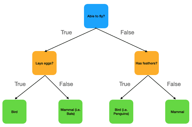
Decision tree learning is a technique used to predict outcomes from discrete (categorical) values. The model represents knowledge in the form of a tree, where each internal node corresponds to a decision based on an attribute, and each branch represents the outcome of that decision. The leaves of the tree indicate the final predicted values.

Once a decision tree is constructed, it can also be rewritten as a set of if–then rules. This alternative form often makes the learned knowledge easier for humans to read and interpret, while still preserving the logic of the original tree.

In general, decision trees represent a disjunction of conjunctions of constraints on the attribute values of instances. Each path from the tree root to a leaf corresponds to a conjunction of attribute tests, and the tree itself to a disjunction of these conjunctions.

Exercise: turning the last image's decision tree into a conjunction-disjunction sentence:

Is able to fly? True: (Bird ^ Lay eggs) v (Bird ^ not(Has feathers)) False: (Mammal ^ not(Lay eggs)) v (Mammal ^ not(Has feathers))

Now let's take a look at the best problems in which we can use decision trees:

• Representation of Instances: in decision tree learning, each element of the dataset is represented using attributes and their values. For instance, an attribute might be Temperature, and its possible values could be Hot, Mild, or Cold. Decision trees are particularly effective when attributes have a limited number of different, non-overlapping values. This makes it easy to create branches in the tree that clearly divide the data into smaller, well-defined groups.

• Handling Different Types of Data: decision trees work naturally with discrete or categorical data, where the outcome belongs to a set of fixed labels. A simple example is predicting whether a person will play tennis on a given day, with possible outputs of Yes or No. Beyond binary classification, decision trees can also handle multi-class problems, where the target has more than two possible values. In addition, some decision tree algorithms are designed to work with numerical attributes. For example, instead of splitting on “Temperature = Hot,” the tree might split on a condition like “Temperature ≥ 30°C.” A more advanced version, known as a regression tree, can even predict real-valued outputs (such as estimating a house price). However, this application is less common compared to classification tasks.

• Expressiveness of Decision Trees: one of the strengths of decision trees is their ability to represent disjunctive descriptions, which means conditions that involve logical “OR” relationships. For example, a decision tree might predict that a person will play tennis if the weather is sunny OR the humidity is low. This flexibility allows trees to represent complex rules in a structured and systematic way, which would be difficult to capture with simple linear models.

• Dealing with Imperfections in Data: decision tree learning methods are robust to imperfect data, which makes them highly practical. If the training data contains errors in classification labels (for example, a day incorrectly labeled as “Play Tennis = Yes”), the tree can still generalize well and make reasonable predictions. Similarly, if there are mistakes in the attribute values (such as recording the wrong temperature), decision trees usually tolerate these errors without a severe drop in accuracy.

• The training data may contain missing attribute values: another common issue in real-world data is missing values. For example, if the humidity is not recorded for certain days, a decision tree can still use the other attributes (such as temperature or wind) to make predictions. Some algorithms even have built-in strategies for handling missing data, such as assigning fractional weights to branches or choosing the most likely value based on the training set.

ID3 Algorithm

ID3 is the acronym of Iterative Dichotomizer 3, which once you understand the algorithm, you realize is pretty self-explanatory.

Dichotomization is the process of dividing something into two completely opposite things. That's what I was referring to: the ID3 algorithm is a iterative algorithm that divides attributes into two different groups to form a tree. Then, it calculates the entropy and information gains of each attribute. This way, the most determinant attribute is put on the tree as a decision node. This process continues iteratively until it reaches a decision.

Now let's do a more in depth analysis of the algorithm:

• The central choice in the ID3 algorithm is selecting which attribute to test at each node in the tree. We would like to select the attribute that is most useful for classifying examples. For this, we are going to use a statistical property called information gain, that measures how well a given attribute classifies the training data. ID3 uses this information gain measure to select among the candidate attributes at each step while growing the tree.

• To calculate the information gain, we use the entropy, which is a measure of uncertainty. It can be calculated as follows $H(S)=-{\sum }_{i=1}^n{p}_i{\log }_2(p_i)$, where $S$ is a collection of examples and $p_i$ is the proportion of examples. Basically, what we are doing here is measuring the bits of entropy (that's why there is as $lo{g}_2$). So a low entropy, let's consider 0, means that the proportion of examples is certain, whilst, a high entropy, 1, means that the proportion is very uncertain.

E.g., a coin with two faces in which both faces are tails has a low entropy because we have the certainty that when tossed, we will be seen tails. While if we have a high entropy, in this case we will have one face with heads and the other with tails. Therefore, once tossed, we will have uncertainty of what is going to come out.

• Once we know all of this, given the entropy of a collection of training examples, we can define the information gain, which is simply the expected reduction in entropy caused by partitioning the examples according to an attribute. We can define it like this $Gain(S,A)=Entropy(S)-{\sum }_{v\in Values(A)}\frac{|S_v|}{|S|}Entropy(S_v)$. Where $A$ is an attribute, $S$ is a collection of samples, $Values(A)$ is the set of all possible values for an attribute $A$ and $S_v$ is the subset of $S$ for which the attribute $A$ has value $v$.

The ID3 algorithm builds decision trees by searching through a space of possible hypotheses to find one that best fits the training data. It starts with an empty tree and gradually adds branches, guided by the measure of information gain, which helps select the most informative attributes. This process is a hill-climbing search that moves from simple to more complex hypotheses without backtracking, meaning it may sometimes settle on a locally optimal tree rather than the global best one.

The hypothesis space of ID3 includes all possible decision trees for the given attributes, ensuring that the target function can always be represented. However, because ID3 maintains only one hypothesis at a time, it cannot compare multiple consistent trees or evaluate alternative solutions. By using all training examples at each step, ID3 makes statistically informed decisions that reduce sensitivity to individual data errors, and with small adjustments, it can handle noisy data effectively.

Example ID3

To make everything clearer and make sure you understand all the steps, I'm going to use a little toy dataset and writte all the steps by hand, so you can see the entire procedure. Usually, people use the "playing tennis outside" dataset, but it is already solved and you have a lot of examples online. So I'm going to use a different one provided by Vidya Mahesh Huddar. Finally, I'm going to code it in python and show you the resolution with code and comparing it with the one we will be doing now. I invite you to do it with me if you understood everything more or less untill this point, and if not, my bad, you can continue reading and solve the exercise later.

In this dataset the objective is to predict if the profit of each candidate is going to be Up or Down. Then, the first step is calculating the entropy of it, so later we can calculate the information gain of each attribute starting from this:

In this case $S=Profit$:

$H(S)=-{\sum }_{i=1}^2{p}_i{\log }_2(p_i)=-\frac{5}{10}{\log }_2\left(\frac{5}{10}\right)-\frac{5}{10}{\log }_2\left(\frac{5}{10}\right)=1$

After that we have to calculate the information gain of the rest of attributes and then select the one with the biggest information gain to keep branching:

• Information gain of age: First, we calculate the entropy of each subset of the attribute: $H(S_{old})=-{\sum }_{i=1}^2{p}_i{\log }_2(p_i)=-\frac{3}{3}{\log }_2\left(\frac{3}{3}\right)-\frac{3}{3}{\log }_2\left(\frac{3}{3}\right)=0$ $H(S_{mid})=-{\sum }_{i=1}^2{p}_i{\log }_2(p_i)=-\frac{2}{4}{\log }_2\left(\frac{2}{4}\right)-\frac{2}{4}{\log }_2\left(\frac{2}{4}\right)=1$ $H(S_{new})=-{\sum }_{i=1}^2{p}_i{\log }_2(p_i)=-\frac{3}{3}{\log }_2\left(\frac{3}{3}\right)-\frac{3}{3}{\log }_2\left(\frac{3}{3}\right)=0$ Then, we calculate the gain using the different entropies: $Gain(S,\text{Age})=H(S)-{\sum }_{v\in \{\text{old},\text{mid},\text{new}\}}\frac{S_v}{S}H(S_v)=1-\frac{1}{10}·0-\frac{4}{10}·1-\frac{3}{10}·0=0.6$

• Information gain of competition: First, we calculate the entropy of each subset of the attribute: $H(S_{Yes})=-{\sum }_{i=1}^2{p}_i{\log }_2(p_i)=-\frac{3}{4}{\log }_2\left(\frac{3}{4}\right)-\frac{1}{4}{\log }_2\left(\frac{1}{4}\right)=0.81$ $H(S_{No})=-{\sum }_{i=1}^2{p}_i{\log }_2(p_i)=-\frac{2}{6}{\log }_2\left(\frac{2}{6}\right)-\frac{4}{6}{\log }_2\left(\frac{4}{6}\right)=0.92$ Then, we calculate the gain using the different entropies: $Gain(S,\text{Competition})=H(S)-{\sum }_{v\in \{\text{Yes},\text{No}\}}\frac{S_v}{S}H(S_v)=1-\frac{4}{10}·0.81-\frac{6}{10}·0.92=0.12$

• Information gain of type: First, we calculate the entropy of each subset of the attribute: $H(S_{SW})=-{\sum }_{i=1}^2{p}_i{\log }_2(p_i)=-\frac{3}{6}{\log }_2\left(\frac{3}{6}\right)-\frac{3}{6}{\log }_2\left(\frac{3}{6}\right)=1$ $H(S_{HW})=-{\sum }_{i=1}^2{p}_i{\log }_2(p_i)=-\frac{2}{4}{\log }_2\left(\frac{2}{4}\right)-\frac{2}{4}{\log }_2\left(\frac{2}{4}\right)=1$ Then, we calculate the gain using the different entropies: $Gain(S,\text{Type})=H(S)-{\sum }_{v\in \{\text{SW},\text{HW}\}}\frac{S_v}{S}H(S_v)=1-\frac{6}{10}·1-\frac{4}{10}·1=0$

Now that we have calculate all the information gains, we choose the attribute age to be the root of out node, since it is the one with the highest gain $0.6>0.12>0$ When we compute the information gain for an attribute, we are measuring how much knowing that attribute reduces the uncertainty about the class. In other words, it tells us how informative that attribute is for predicting the target.

A higher information gain means that the attribute provides a better separation of the training examples into groups that are more “pure”, meaning that most examples in those groups belong to the same class. This helps the algorithm make more confident and accurate predictions.

The ID3 algorithm follows a greedy strategy, meaning that at each step, it chooses the attribute that seems best at that moment. By using the most informative attribute at the root, ID3 ensures that the first split divides the dataset in the most meaningful way possible. This leads to a simpler and more efficient tree because early splits quickly reduce uncertainty. Each subsequent node then repeats the same process on its subset of data until the tree is complete.

The tree for the moment is going to look like this, with the attribute Age as root and its values as branches:

graph TD
    A[Age] -->|old| B
    A -->|mid| C
    A -->|new| D

Now we have to look at each branch and repeat the las process but with the specific subset of examples which contain that certain Age as attribute. But if we look carefully to the data, we can save several minutes of work, becase it can happen that the final answer is already in the data:

Here, if the Age is Old, doesn't matter the rest of attributes, because the profit is going to be Down every time.

The same happens with the Age being New, the profit is going to be always Up. This way, we can generalize the answers and say that if the candidate is Old, the profits are Down and if the candidate is New, the profits are Up.

graph TD
    A[Age] -->|old| Down
    A -->|mid| C
    A -->|new| Up

Then we end up with this data, in which we have to repeat the same process as before, but with one attribute less. If in other datasets, we aren't this lucky, we will have to split the data into these subsets and calculate everything again, as we are going to do now.

Now, the entropy to compare with is going to be the elements with the Age being Mid $S=S_{mid}$. We have already calculated it in the last step, but I rewrite it as a reminder:

$H(S_{mid})=-{\sum }_{i=1}^2{p}_i{\log }_2(p_i)=-\frac{2}{4}{\log }_2\left(\frac{2}{4}\right)-\frac{2}{4}{\log }_2\left(\frac{2}{4}\right)=1$

And we recalculate the information gains:

• Information gain of competition: First, we calculate the entropy of each subset of the attribute: $H(S_{Yes})=-{\sum }_{i=1}^2{p}_i{\log }_2(p_i)=-\frac{2}{2}{\log }_2\left(\frac{2}{2}\right)-\frac{0}{2}{\log }_2\left(\frac{0}{2}\right)=0$ $H(S_{No})=-{\sum }_{i=1}^2{p}_i{\log }_2(p_i)=-\frac{0}{2}{\log }_2\left(\frac{0}{2}\right)-\frac{2}{2}{\log }_2\left(\frac{2}{2}\right)=0$ Then, we calculate the gain using the different entropies: $Gain(S_{mid},\text{Competition})=H(S)-{\sum }_{v\in \{\text{Yes},\text{No}\}}\frac{S_v}{S}H(S_v)=1-\frac{2}{4}·0-\frac{2}{4}·0=1$

• Information gain of type: First, we calculate the entropy of each subset of the attribute: $H(S_{SW})=-{\sum }_{i=1}^2{p}_i{\log }_2(p_i)=-\frac{1}{2}{\log }_2\left(\frac{1}{2}\right)-\frac{1}{2}{\log }_2\left(\frac{1}{2}\right)=1$ $H(S_{HW})=-{\sum }_{i=1}^2{p}_i{\log }_2(p_i)=-\frac{1}{2}{\log }_2\left(\frac{1}{2}\right)-\frac{1}{2}{\log }_2\left(\frac{1}{2}\right)=1$ Then, we calculate the gain using the different entropies: $Gain(S,\text{Type})=H(S)-{\sum }_{v\in \{\text{SW},\text{HW}\}}\frac{S_v}{S}H(S_v)=1-\frac{6}{10}·1-\frac{4}{10}·1=0$

As the information gain in competition is the maximum possible, we choose it over the type.

$1>0$

Now the tree would be looking like this:

graph TD
    A[Age] -->|old| Down
    A -->|mid| Competition
    A -->|new| Up
    Competition -->|yes| B
    Competition -->|no| C

So we look at the data again to see if we can see the answer or if we need to keep calculating:

And luckily, we reached a conclusion: if the candidate has the attribute competition, the profit is going to be Up. In the opposite case, the profit is going to be Down. Therefore, we have reached some leaf nodes, and we don't need nothing else to compare. Finally, the tree is going to look like this:

graph TD
    A[Age] -->|old| Down 
    A -->|mid| Competition
    A -->|new| Up 
    Competition -->|yes| Down
    Competition -->|no| Up

So the solution to this problem is the following:

Up: (not(competition) ^ mid) or new Down: (competition ^mid) or old

Code ID3

Now let's take a look at the python code. I will explaing everything step by step, but focusing on the theory and not how python works itself.

class TokenType(Enum):
    LParen = "LParen" # (
    RParen = "RParen" # )
    NotOp = "NotOp" # !
    AndOp = "AndOp" # &
    OrOp = "OrOp" # |
    ImpliesOp = "ImpliesOp" # ->
    BiconditionalOp = "BiconditionalOp" # <->
    Variable = "Variable" # A-Z Upper case
    Eof = "Eof" # The endline character (depends on stdin)

CART Algorithm

CART is the acronym of Classification And Regression Tree

Example CART

To make everything clearer and make

Code CART

Now

Conclision

We have now reached the end of the tutorial! And although it is not the most complex example, it still shows the power of the interpreter and how it can be used to evaluate any kind of computation.

As always, thanks for reading and if you have any questions or comments feel free to reach out to me on X/Twitter or by mail at davidvivarbogonez@gmail.com, I am always open to criticism, just like I hope you did by reading this, I am always trying to learn and improve.

Also, as a bonus, you can find a version of this project in F# in github.com/4ster-light/f-logic, for those who are interested and wanna expand their learning further, you will find interesting ways that Functional Programming helps in this kind of problems, as well as algebraic data types, discriminated unions, pattern matching, etc.

References

[4] (ML 2.1) Classification trees (CART). YouTube, https://www.youtube.com/watch?v=p17C9q2M00Q, 2024.
[5] (ML 2.2) Regression trees (CART). YouTube, https://www.youtube.com/watch?v=zvUOpbgtW3c, 2024.